INTRODUCTION
The self-driving car is a rapidly growing technology in today’s ever advancing world. The application may, however, see as an interesting and bridging the gap between humans and machine the tech is yet not complete.
This post will mainly focus on how the entire algorithm works, this will include explanations of deep neural networks, including convolutional neural network, computer vision, and integrating sensor information.
For practical demonstration of the algorithms I will be building an autonomous car using udacity self-driving car simulation which is built in unity. The algorithm I will make will try to learn from my driving patterns and then finally learn from it and drive own its own on any track.
Along with a controlled driving it is also necessary to follow the traffic signs and alter the driving patterns accordingly. A street sign recognition system will also be discussed in this post.
Finally for better performance by the AI, advance lane detection algorithm using computer vision will also be discussed in the post.
The applications/system specs:
- Using google collab for computation (using GPU for run time service).
- Programming language used: python
- Framework: keras(running tensorflow in the backend)
- Libraries: keras, sklearn, opencv, matplotlib, pandas, flask, socket-io, imgaug, numpy, os.
- Simulator: Udacity self-driving car simulator.
- Operating System: Ubuntu
SIMPLE LANE DETECTION.
For making a lane detection algorithm the following python packages were imported:
- python open cv for augmentation and manipulation of computer vision
- numpy for matrix manipulation and calculation.
- matplotlib.pyplot for plotting and displaying images.
Canny edge detection:
i) The first part of the algorithm is applying the canny edge detection function to the image:
The canny edge detection algorithm works according to the bellow procedures.
- First, the noise in the image is removed by using the Gaussian filter to smoothen the image.
- Find the intensity gradients of the image.
- Apply non-maximum suppression.
- To determine the edges double threshold is applied.
- Apply the hysteresis thresholding while using the open cv canny function we will have to pass in values to the minVal and maxVal(names of the variable) of intensity gradient which are used in this stage.
Those pixel intensities of the image that are below the minVal are considered to be non-edges and are so discarded, any value above the maxVal are considered sure to be an edge, while any value between maxVal and minVal are classified as edges or non-edges based on their connectivity. If they are connected to the “sure-edge” pixels, they are considered to be part of the edge otherwise they are discarded.
ii) Define a function canny taking one single argument image which will be an array of different intensity of RGB pixels in the image
iii) Now convert the input image to grayscale this will reduce the image noise by converting the 3 channel image into 2 channel one. By using open cv this can be easily achieved by using the open cv library of python:
cv2.cvtColor(image, cv2.COLOR_RGB2GRAY)

iv) Apply the gaussian blur to the grayscale image to smoothen the image out. Use open cv GaussianBlur function with a kernel size of (5, 5):
cv2.GaussianBlur(image,(5,5), 0)
v) Finally apply the canny function to get the edge value of the image. Use canny function from open cv library, in it the first argument will be our input image, then second and third argument as discussed above are minVal and maxVal.
vi) Then return the edge detected image

CREATE IMAGE REGION OF INTEREST:
i) The first step to creating the region of interest of image is to visualize the image using matplotlib in windowed mode. First read the required image from the image_path using matplotlib.image.imread(<image_path>) and the display the image using matplotlib.image.imshow(image).
From the image markdown the points of quadrilateral on the region where the road is.
ii) Now make a function taking one argument of image to compile all the algorithms in one package.
iii) Make a mask with all pixel values in the image as (0,0,0), this can be easily done by using
numpy.zeros_like(image)
iv) Now make white window by using the coordinates we took before and filling the inside by with white color. This can be achived by through the following command.
cv2.fillPoly(mask, polygons, 255)
v) Now we will take out all the edges of the image that are enclosed by the window.This can be done using the following script:
masked_image=cv2.bitwise_and(image, mask)
vi) Now return the masked image
MAKE LINES:
Open cv makes our lives much easier with its HoughLinesP function:
Lines=cv2.HoughLinesP(cropped_image, thickness, numpy.pi/180, 100, numpy.array([]), maxLineGap=5)
AVERAGE SLOPE INTERCEPT:
i) Make a function which will be taking image and lines from before.
ii) Make 2 lists left_fit, which will hold coordinates of the left line and right_fit which will hold the values of right line.
iii) Iterate through each line in lines and follow the bellow procedure.
iv) Separate the coordinates of stating point and ending point from each line into x1, y1 and x2, y2 respectively.
v) Now pass these coordinate values in the linear polynomial equation Y=mX+c, this equation will help us to derive the slopes and intercepts
vi) Now check if the slope is less than 0, then that slope and intercept value will belong to left line so we will append those values to the left_fit, else otherwise the slope and intercept belong to the right line and so we will append these values to the right_fit.
vii) Now exit the loop and average out the values in left_fit list and right_fit list independently into left_fit_average and right_fit_average respectively.
viii) To get the coordinates for these lines follow the mathematical steps:
->Firstly the y1 will be the height of the image
y2=y1 X (3/5)
x1 = (y1 – intercept) / slope
x2 = (y2 – intercept) / slope
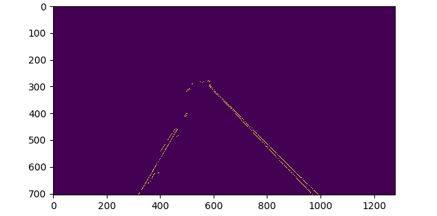
DISPLAY LINES
To display the so build lines first make a function which will be taking first argument as image and second argument as averaged out line coordinates from the previous step.
Firstly make the input image completely black, as discussed above.
Iterate through each line in lines and then separate out the coordinates x1, y1, x2, y2 from each line. Then finally draw a line using open cv line function which would be taking its argument as the blackened image, second and third argument as starting and ending point respectively, fourth argument as the color of the lines and final fifth argument as thickness of the line.

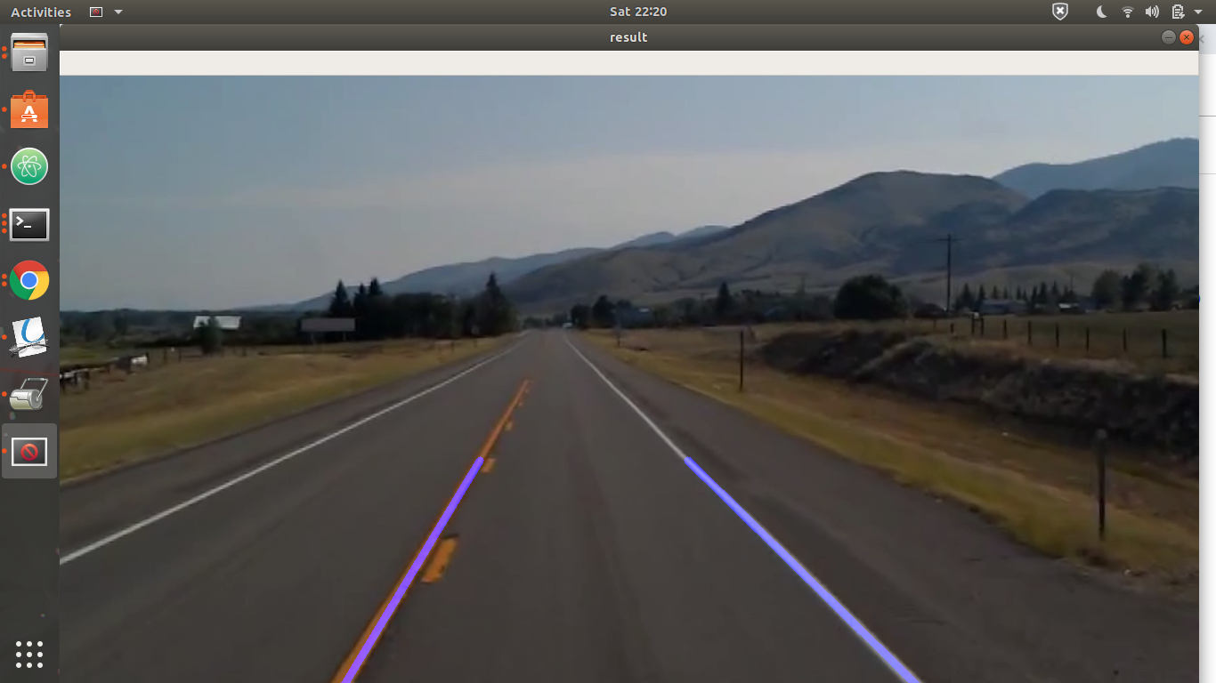
CREATING THE COMBO IMAGE
Now we will combine the above-created line image with the actual image. This can be easily be done by using the open cv addWeighted function
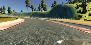
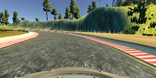
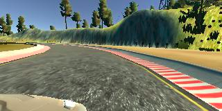
ABOUT UDACITY SELF DRIVING CAR SIMULATOR.
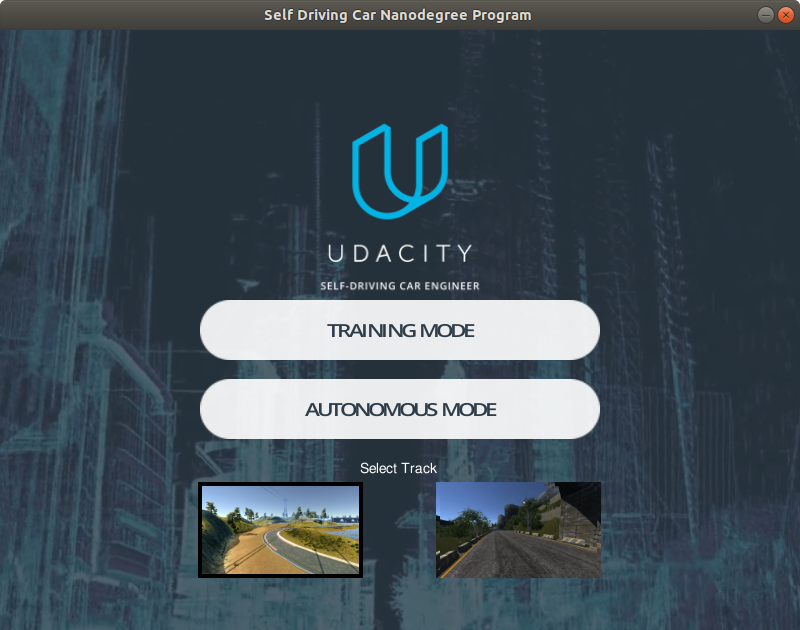
The udacity self-driving car simulator was built on unity game engine. This simulator was built as a part of udacity self-driving car nano degree program.
The simulator has car simulation has 3 cameras to record middle left and right sides of the car. To prepare the training data, the simulator is run on the training mode. In the training mode, the car can be controlled with W, A, S, D or by using arrow keys.
Data will start collecting on pressing the record. To prepare a good model follow the following simple rules:
- The car should mostly be made to run at the center of the track.
- Try some times to deviate from the center of the track to either side in an attempt to crash and then regain the position back to the center. This data is necessary to teach the car how to regain its control after losing control and going off track.
- Take a minimum of 3 laps around the track in one particular direction. Then take 3 laps in the reverse direction. This is done because in the first 3 laps our car is taking a lot of left turns and very less right turn even this out we make our car run in the opposite direction to get an adequate amount of data to work on.
On ending the recording process the image files are stored in the defined path with a CSV file which contains the required image path and the corresponding steering angles.
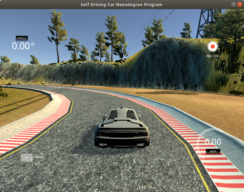
Once you have prepared your AI model and an application to make the client to server connection. you have to run the simulator on autonomous mode.
BEHAVIORAL CLONING
GATHERING AND BALANCING THE DATA
To explain the algorithm ill be taking the entire process step by step.For this algorithm, I was using pandas library to read the csv file and apply a slight alteration to the collumn data.
To get started first get the data from the CSV file created by the emulator using pandas.read_csv(). Trim the image paths to just image names.

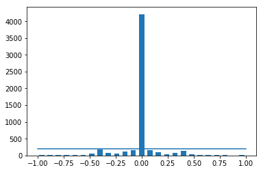
Fig: The above representation shows that 0 degree angle has the maximum frequency.
The above representation makes it clear that the frequency of 0-degree angle is the way to high compared to the rest. This happened because of our attempt to create a stable vehicle. Now if allow our model to learn on this dataset it will not make any turns and will just move straight to prevent this we will make threshold value (in this case 200) then we will randomly take the steering values by shuffling our dataset. This shuffling ensures that we have data around the track and not just starting few. Now by plotting the bar graph, it can be observed that the straight path is in alignment with the rest of the steering angles. 
Fig: Frequncy reprensentation after applying a threshold of 200 images.
Now make a function to iterate through each of 200 image paths and load their steering angles and append them sequentially according to the image paths to a list steering_angles.
This process of limiting the data is important to enhance the training of the model.
SEPARATE INTO TRAINING AND VALIDATION SETS:
Now in this step like the heading says we have to split our data set of 200 image paths and steering angles into training and validation sets. This will further help us limit the time taken to apply our data manipulation to the training set only and not on the entire data set.
Separation of training and validation sets can be achieved by using the function test_train_split from sklearn.model_selection library which will take the first argument as independent variable, second argument as the dependent variable, Third argument as test_size which we will keep as 20% of the total dataset which is 40 and finally the fourth argument is the value to the random_state this will give us a fixed value to our training and validation sets no matter how many times we run this code line.
X_train, X_valid, y_train, y_valid=train_test_split(imge_paths, steerings, test_size=0.2, random_state=6)
VISUALISATION OF DATA IN TRAINING AND VALIDATION SETS
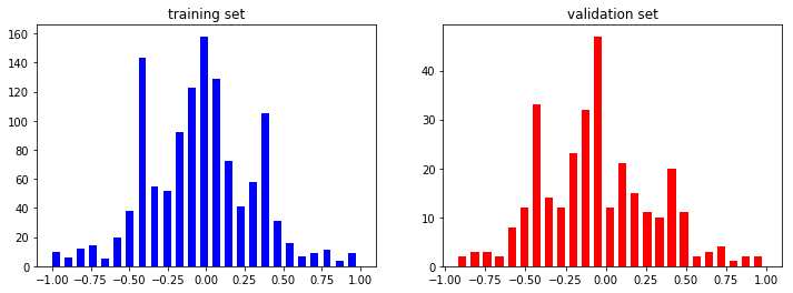
Fig: The above figure shows frequency of ech angles in training and validation set.
IMAGE AUGMENTATION
i) First image augmentation algorithm we will use is simply to zoom the image.
a) Make a function zoom which will be taking in a single input of image value.
b) For zooming, we will be using affine function from imgaug which will take in a single argument of scale which is the range within which the input image will be zoomed. Make an object zoom of this function with scale value ranging from 1 to 1.3.
c) Now to augment this object on the image call in the function zoom.augment_image with an argument image.
iii) Random brightness
a) Make a function zoom which will be taking in a single input of image value.
b) For zooming, we will be using affine function from imgaug which will take in a single argument of scale which is the range within which the input image will be zoomed. Make an object zoom of this function with scale value ranging from 1 to 1.3.
zoom=augmenters.Affine(scale=(1, 1.3))
c) Now to augment this object on the image call in the function zoom.augment_image with an argument image.

Fig: Image augmentation: zoom

Fig; Image augmentation: panning
iii) Random brightness
Make a function which will take in a single argument as image
For applying brightness to the image we will use Multiply function from imgaug it can increase decrease the brightness of the image.
The Multiply function will take in a single argument of the range within which the image is to be dimmed or brightened.
In this case we will take in a range from 0.2 to 1.2 here 1 is considered to be in original brightness of image. Define brightness as the object of this function.
Finally augment this object on the image.
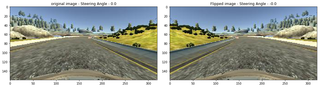
iv) Random flip
a) Make a function which will take in 2 arguments of image and steering_angle
b) For flipping the image this can be achieved by using flip function from open cv which will take in first argument as image and the second argument as flipCode here we are using 1 which means flipping around Y-axis
c) Negate the steering_angle to always get the angle after flipping over 180 degree.
d) return both the values.
v) Random image augmentation
a) Make a function which will take in 2 arguments as image path and steering angles as inputs
b) This function will communicate and call the above made image augmentation functions at random
c) The randomness is dependent on the on the random.rand function which is passed through an if condition every time and is checked if it is less than 0.5, then it executes the function under it.
d) Finally return the image and steering_angles


On the basis of the loss function shown above it can be noted that validation and training plots decreases over epochs also the the validation line never overlaps the training hense it can be said that our so we made a generalized model for our simulated car.
F. CONNECTING THE MODEL TO THE SIMULATOR:
i) The Udacity self-driving car simulator passes the image over to the server at port 4567, it also listens the steering and throttle information from the server. Knowing this we have to make client to server and server to client connection. This whole process is made simple by making use flask, socket io libraries.
ii) Make a new python script application for server-client connection. Follow the below steps to make this work.
a) We will be using flask application which acquires server connection, besides this we will also be using socketio for server to client communication for sending the steering and throttle information.
b) Load the model that we saved earlier using the keras library connect the flask application with the socketio, and establish a server connection at 4567
i.e. `model=model.load(‘model.h5’)
app=socketio.Middleware(socketio.Server, app)
eventlet.wsgi.server(eventlet.listen((‘’, 4567)), app)`
c) Make a function to send controls to the simulator, taking both steering angles and throttle values as input and by making the use of emit function of socketio send steering angle and throttle values as dictionary values.
i.e. `sio.emit('steer', data = {
'steering_angle': steering_angle.__str__(),
'throttle': throttle.__str__()
})`
d) Test if the connection is established. Make a decorator, which fires up a connect function only when the connection is established try printing ‘Connected’ and try sending a hardcoded value to send the values to the function which is sending information to the server. Check the simulator and the terminal if we have the required outputs.
e) Once the above test is successful make another decorator which fires up the telemetry function when it receives the image data.
f) Extract the image from the server and decode it using the b64decode function from base64
g) Convert the image data to numpy array type, and pass the image through the image_preprocess function similar to as made earlier
h) Now using this image ,predict the steering angle in float values.
i) Outside the function declare a speed limit with value of 10, and calculate the throttle according to the following formula.
-> throttle = 1.0 – ( speed / speed_limit )
This will maintain a proportional throttle with respect to speed.
j) Finally send these steering angle and throttle values to the simulator by calling send_control function.
The Multiply function will take in a single argument of the range within which the image is to be dimmed or brightened.
In this case we will take in a range from 0.2 to 1.2 here 1 is considered to be in original brightness of image. Define brightness as the object of this function.
Finally augment this object on the image.
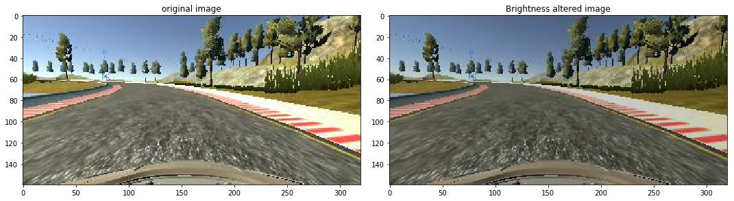
Fig: Image augmentation; Random brightness
iv) Random flip
a) Make a function which will take in 2 arguments of image and steering_angle
b) For flipping the image this can be achieved by using flip function from open cv which will take in first argument as image and the second argument as flipCode here we are using 1 which means flipping around Y-axis
c) Negate the steering_angle to always get the angle after flipping over 180 degree.
d) return both the values.
Fig; Image augmentation; image flip
v) Random image augmentation
a) Make a function which will take in 2 arguments as image path and steering angles as inputs
b) This function will communicate and call the above made image augmentation functions at random
c) The randomness is dependent on the on the random.rand function which is passed through an if condition every time and is checked if it is less than 0.5, then it executes the function under it.
d) Finally return the image and steering_angles
Fig: Random combination of above mentioned image augmentation methods.

Fig: After applying the image preprocessing on training and validation images.
E. CREATING AN AI MODEL
Before creating an AI model we have to start by creating a generator that will be used to process and augment data through all the above mentioned functions at a particular batch size. Thereby saving a lot of time over preparing the data for training the AI
i) Creating batch generator:
a) Firstly a generator function allows you to declare a function that behaves like an iterator and let you use it in a for loop. The difference between an iterator and a regular function is that after we return a value the program destroys all the variable created in the function, but this is not the case in generator, when generator yields a value at the end of the function it keeps the information of the variable in the memory for if the function is to recalled again.
b) Make a function named batch_generator accepting the arguments of image paths, steering angles, batch size and a Boolean variable to separate the changes over training and validation.
c) Start an infinite loop, and declare an empty list bath_image and batch_steering which will contain the set of images and steering angles in quantity of a particular batch size.
d) Initialize a for loop in the range of the particular batch size and then declare an object to hold peculiar random integer between 0 and length of the list of image paths passed as an argument
i.e. `random_index=random.randint(0, len(image_paths))`
e) Pass an ‘if’ condition to check if the generator is used for training or for validation. If a the condition is true pass the image paths and steering angles at index=random_index through the random_augment function as discussed above.
Else just read the same image and same steering angles.
f) Now exit the if conditions and pass the output image through the image_preprocess function, and append the batch_img and batch_steering with the output image and the steering angles.
g) Yield the batch_img and batch_steering.
ii) Creating CNN model
a. For building the AI using deep neural net we will use the keras library which will run tensorflow in the backend
b. Make a function to hold the neural net
c. Initialize the model by making an object of Sequential class.
i.e. `model=Sequential()`
d. Add a convolution 2d layer with 24 filters, and convolution layer of size (5,5), this convolution matrix will move horizontally and vertically at 2 units per iteration in each, pass in the input shape of the image in the format (height, width, and number of channels of the image), and specify the activation function in this case we will be using exponential linear unit or as the abrevation ‘elu’.
i.e. `model.add(Convolution2D(24, 5, 5, subsample=(2,2), input_shape=(66, 200, 3), activation=’elu’))`
e. Add the second convolution 2d layer with 36 filters and convolution layer of size (5,5), and with the same subsample and activation function note this time we will not be specifying the input shape as it was already specified before.
i.e. `model.add(Convoloution2D(36, 5, 5, subsample=(2,2), activation=’elu’))`
f. Add the third convolution 2d layer with 48 layers and keeping the rest of the argument same as in step ‘e’
i.e. `model.add(Convoloution2D(48, 5, 5, subsample=(2,2), activation=’elu’))`
g. Add the fourth and fifth convolution 2d layer with the same no of filters of 64, convolution matrix size of (3,3), and with the activation function ‘elu’
i.e. `model.add(Convolution2D(64, 3, 3, activation=’elu’))`
h. Add a 50% dropout layer, this will deactivate ½ of the unused neurons in the neural net helping to prevent overfitting of the model
i.e. `model.add(Dropout(0.5))`
i. Add a flttening layer to flatten out the images to convert the 2 dimentional image matrix to one dimentional one to feed these values as the input values to the neural net.
j. Now to make the hidden layers in the deep neural net, add a Dense layer with 50 output nodes and with the activation function ‘elu’.
k. Now add the second hidden layer with of the neural net by adding a Dense layer with 10 output nodes and with the activation function ‘elu’.
l. Finally make the output layer of the neural net by adding the Dense layer with a single output node.
m. Now for making a fully connected neural net we have to compile the using the Adam optimizer, with a learning rate of 10-4, and with loss function of mean square error
i.e.`model.compile(loss = ‘mse’, optimizer = Adam(lr=1e-4), metrics = [‘accuracy’])`
iii) Understanding the deep neural net so formed:

Fig: Summary of the Self-driving car model
As it is clear from above observation the total number of parameters to be trained is 252219
iv) Training the model:
a) For training the model we are going to use the fit generator function so that each time the input is called from the generator we created earlier.
b) Inside model.fit_generator, the first argument we are going to pass is our generator function in which we the inputs as X_train and y_train, created before, we are going to pass these values over a batch size of 100, in training model.
i.e. `batch_generator(X_train, y_train, 100, 1)`
We are going to iterate through the entire dataset over 10 epochs.
c) validation data we are again going to pass our validation sets through our batch_generator with is training arguments as false. Finally we will shuffle our dataset over each iterations.
i.e. `history=model.fit_generator(batch_generator(X_train, y_train, 100, 1), steps_per_epoch=300, epochs=10, validation_data=batch_generator(X_valid, y_valid, 100, 0), validation_steps=200, verbose=1, shuffle=1)`
v) Analysis of the trained model:
Fig: The above figure shows the decrease of loss value of validation and training with the increasing number of epochs.
On the basis of the loss function shown above it can be noted that validation and training plots decreases over epochs also the the validation line never overlaps the training hense it can be said that our so we made a generalized model for our simulated car.
F. CONNECTING THE MODEL TO THE SIMULATOR:
i) The Udacity self-driving car simulator passes the image over to the server at port 4567, it also listens the steering and throttle information from the server. Knowing this we have to make client to server and server to client connection. This whole process is made simple by making use flask, socket io libraries.
ii) Make a new python script application for server-client connection. Follow the below steps to make this work.
a) We will be using flask application which acquires server connection, besides this we will also be using socketio for server to client communication for sending the steering and throttle information.
b) Load the model that we saved earlier using the keras library connect the flask application with the socketio, and establish a server connection at 4567
i.e. `model=model.load(‘model.h5’)
app=socketio.Middleware(socketio.Server, app)
eventlet.wsgi.server(eventlet.listen((‘’, 4567)), app)`
c) Make a function to send controls to the simulator, taking both steering angles and throttle values as input and by making the use of emit function of socketio send steering angle and throttle values as dictionary values.
i.e. `sio.emit('steer', data = {
'steering_angle': steering_angle.__str__(),
'throttle': throttle.__str__()
})`
d) Test if the connection is established. Make a decorator, which fires up a connect function only when the connection is established try printing ‘Connected’ and try sending a hardcoded value to send the values to the function which is sending information to the server. Check the simulator and the terminal if we have the required outputs.
e) Once the above test is successful make another decorator which fires up the telemetry function when it receives the image data.
f) Extract the image from the server and decode it using the b64decode function from base64
g) Convert the image data to numpy array type, and pass the image through the image_preprocess function similar to as made earlier
h) Now using this image ,predict the steering angle in float values.
i) Outside the function declare a speed limit with value of 10, and calculate the throttle according to the following formula.
-> throttle = 1.0 – ( speed / speed_limit )
This will maintain a proportional throttle with respect to speed.
j) Finally send these steering angle and throttle values to the simulator by calling send_control function.
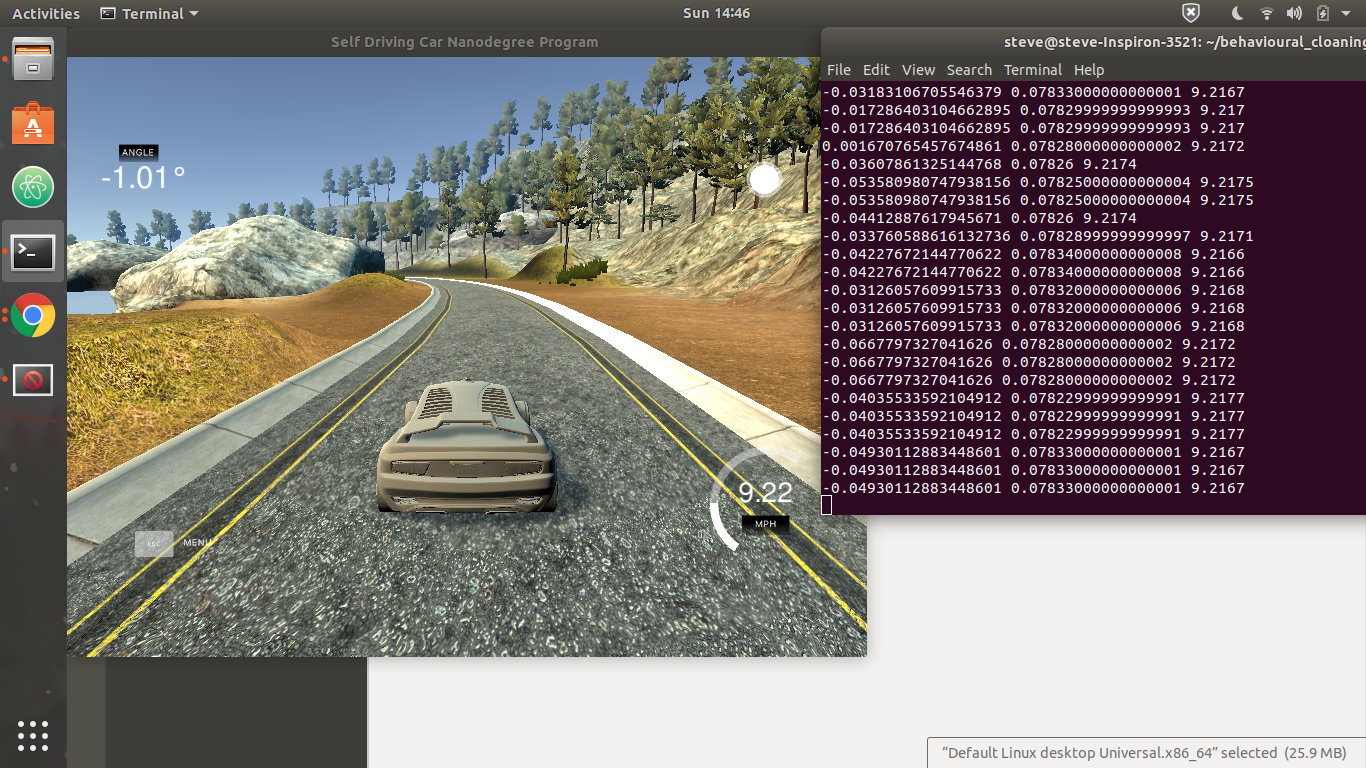
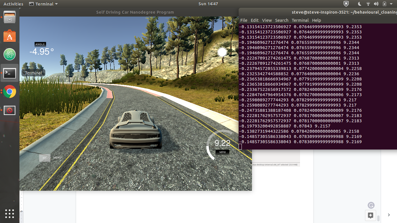
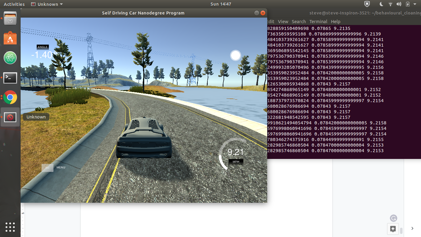
Fig: The above figure shows how model is working flowlessly in the simulated static environment.
Comments
Post a Comment